The data have been processed to 32 bit floating point image format from the raw interferograms collected by the FTHSI. The image is unwarped, but has been through a destreaking routine. Chuck Rhode and Wil Slough performed the MTU portion of the processing.
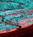
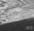
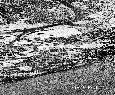
Figure 1 is an RGB image, with red=594 nm, green=695 nm and blue=810 nm. The wavelengths were selected (somewhat non-systematically) to produce an interesting color image. The annotation on the image refers to locations of spectra acquired for visually distinct feature classes in the image (e.g., pavement, water, sand, etc.). These six spectra are graphed in Figure 2.
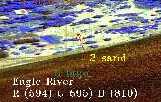 Figure 1: Eagle River RGB Image
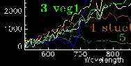 Figure 2: Spectral Plots of Figure 1 Features
PC band images
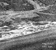
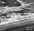
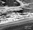
Figure 3 below is 9 images selected at 10 band intervals from the eag1t data set. Each image was contrast enhanced using the ENVI Quick Enhancement > Equalization function.
The purpose of this image set is to
- show the manner in which features change their reflectivity with wavelength,
- how contrast between features changes with wavelength
- how noise decreases from lower to higher wavelengths. The system and detector are less sensitive at the blue end of the spectrum, hence the signal to noise ratio decreases.
Figure 3.
 RGB 645/810/916 nm
 527 nm
 553 nm
 587 nm
 624 nm
 667 nm
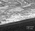 715 nm
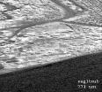 771 nm
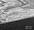 837 nm
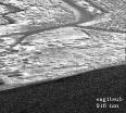 916 nm
 1010 nm
Principal Components Transformation
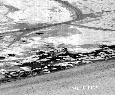
Figure 4 is an image comprised of principal components (PC) bands 1,2 and 3 in red, green and blue. Next, the individual bands (PC1, PC2, PC3) are shown as greyscale images. An eigenvalue plot (Figure 5) shows the relative loading of each PC band, indicating that the bulk of the information is concentrated in the first three or four bands. Animation of images of all 91 PC bands supports this; PC bands 5-91 appear noisy (e.g., high degree of speckle), as might be expected. Note that all 91 available bands were input into the PC transform, including the originally noisy channels in the blue region. Hence, noise (low SNR) due to low photon flux in the blue wavelengths was incorporated directly into the transform. Omitting noisy bands from input to the PC transform may improve the output.
Figure 6 is similar to Figure 4, differing in that the PC 123 image have been processed using ENVI's Decorrelation Stretch function.
Principal Components Images
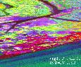 Figure 4: PC 123
 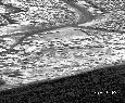 PC 1
PC 1
 PC 2
PC 2
 PC 3
PC 3 PC 213
Eigen value loadings relating to distribution of information among the PC bands.
 Figure 5: Eigenvalue loadings of Principal Components
PC image with decorrelation stretch
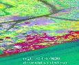 Figure 6: PC 123 with decorrelation stretch applied
(Note: these are preliminary data. They have not yet been flat fielded, dark current subtracted, destreaked or georectified.)